
[Georg Nees (1926-2016) is known as a pioneer of computer art, in a profoundly exciting time when mathematics blended seamlessly with art, and computational aesthetics was first being theorized. These ideas were confronted by a milieu of thinkers who today are largely unknown in the English-speaking world — notably Max Bense, to whom this paper was dedicated. The present paper is a tutorial introduction to denotational semantics of programming languages, viewed through the lens of Peircian semiotics. We might think of it as a step up from a certain deeply mediocre book on the semiotics of programming — and written in 1980 no less. Edits to the translation are welcome.]
1. Introduction
In the domain of C.S. Peirce we bring together the work of two thinkers: Max Bense and Dana Scott. Bense is familiar to us, Scott perhaps less so: he received his Ph.D in 1958 and is now Professor of Mathematical Logic in Oxford, England. As an example of his range, refer to [1]. What we are discussing began in 1969 as a collaboration between Scott and computer scientist Christopher Strachey, who died in 1975 ([2,3,4]). We can only mention in passing the influence of Lawvere ([5]).
Strachey and Scott were looking for mathematical semantics for programming languages. However, Scott noticed that this question was overshadowed by a more complicated and until then largely unsolved problem, namely, efficient models of λ-calculus ([6,7]). The models that Scott found have a peculiar analogy to real analysis; indeed, they contain rational and transcendental elements ([8]). Scott built a new type of information theory into his semantics ([8,9]).
Programs can be viewed as imperative clauses or texts, since they are commands to entities. We pick out a subclass from these texts, namely programs, which in turn process texts. From a semantics of text processing we then try to proceed to a Peirce/Bense/Scottian semiotics of text processing. As a follow-up, we list a few epistemological questions.
2. Text Processing
Now let’s learn to program! We imagine a word processing machine that has drawers (memory cells). The first 17 drawers are labeled \(a\) through \(r\). Then follow \(s\), \(t\), \(u\), \(v\), \(w\). Then follow 1000 drawers each: \(x_{\tiny 1}\), ..., \(x_{\tiny 1000}\), \(y_{\tiny 1}\), ..., \(y_{\tiny 1000}\), \(z_{\tiny 1}\), ..., \(z_{\tiny 1000}\). There is a note with a number in each of the drawers \(a\) to \(r\). In all the other drawers there are notes (books) on which a text is written. In technical reality, drawers are replaced by, say, magnetic disks. As variables for cells (drawers) we choose names with at least two characters, e.g. xx or Text4. Our text processor can do the following basic operations:
\1 Text1 := Text2             -- text in cell Text1 is replaced with a copy of the text in cell Text2
\2 head(Text1)                -- get first symbol of text in Text1
\3 tail(Text1)                -- get all symbols except the first in Text1
\4 print(Text1), read(Text1)
Notice that we need not make a strict distinction between cells and text, because one also says “Please bring the SEMIOSIS folder” to mean the text in that folder. Application example for /1 ... 3:
/5 Ta := head(tail(tail("Tony Meier, male, born 02.03.01")))This triggers the storage of the symbol ‘male’ in cell Ta. As text symbols, we allow words and the special characters “.,;!?” too. The following combination principles for basic operations are (just like /1, 4) commands (instructions) to the computer:
/6 while B do C        -- as long as B holds, do C
/7 if B then C else D  -- if B holds, do C, otherwise do D
/8 C1; C2; ... ; Ck    -- do C1, C2, ..., Ck in sequence
Application example! Suppose in \(x_{\tiny 1}\), ..., \(x_{\tiny 1000}\) personnel files are based on the scheme of the innermost bracket in /5. Then the following program lists the files of all males with surname “Meier”:
/9.1 n:=1; while n≤1000 do
  .2 (if head(tail(tail(Xn))) = "male"
  .3 and tail(tail(Xn)) = "Meier" print Xn else dummy)
In /9.2, dummy is the dummy operation that does nothing. Here our text processor serves as a personnel database. Surely we all realize how powerful it can be made by layering code on top of itself in a building-block fashion.
3. Text Semantics
Now we have to make friends with mathematics! Our programs are themselves texts. What is the meaning (the object reference) of these texts?
We start with the concept of function. A function (mapping, morphism) \(f\) maps the elements of a set \(S_d\) (domain of \(f\)) to elements of a set \(S_r\) (range of \(f\)). One writes:
\[f(S_d) = S_r \;\;\mathrm{or}\;\; f : S_d \to S_r \;\;\mathrm{or}\;\; S_d \xrightarrow{f} S_r\]
Morphisms (functions) are also called arrows. They are members of categories, but that doesn’t matter right now (Lawvere!). If \(S_f\) is a set of family names, \(S_g\) a set of given names, let \(f\!f\!g\) be the arrow that assigns to each surname \(\in\) (in) \(S_f\) a set of first names \(\in 2^{S_g}\); here \(2^{S_g}\) is the set of subsets (power set) of \(S_g\). A single assignment is denoted by a single arrow, as follows:
\[\mathrm{Rilke} \;\xrightarrow{ffg}\; (\mathrm{Rainer}, \mathrm{Maria}) \in 2^{S_g}\]
The set of all mappings \(f\) from a set \(S_1\) to another \(S_2\) is called a morphism space \(mor(S_1,S_2)\). If \(S_1 = S_2\), then the morphisms are called endomorphisms.
We now make a surprising statement: the meaning of a command (see 1/1,4,6,7,8) is an endomorphism of the text processor’s memory. We can digest this step by step: strictly speaking, it is an endomorphism of the space (set) of memory states. A memory state is a function
\[\mathrm{Cells} \,\xrightarrow{z}\, \mathrm{Text}\]
which tells you which text is in which drawer. A change of state \(a\) is then an arrow afterwards:
\[(\mathrm{Cells} \,\xrightarrow{z_1}\, \mathrm{Text}) \,\xrightarrow{a}\, (\mathrm{Cells} \,\xrightarrow{z_2}\, \mathrm{Text})\]
This is clearly the transition \(a\) from a state \(z_1\) to a state \(z_2\). However, a command is still more. Let’s look at the assignment command (cf. /1)
\[\mathrm{Text}_1 := \mathrm{Text}_2\]
Although this assignment only changes the contents of a single drawer, the effect on the overall memory depends on the initial state. So the meaning of := is an arrow
\[mor(\mathrm{Cells},\mathrm{Text}) \,\xrightarrow{f}\, mor(\mathrm{Cells},\mathrm{Text})\]
What is this endomorphism \(f\)? It is the object of the object reference whose sign is the program text (carefully set in quotation marks) ‘Text1 := Text2’.
The object reference must in turn be produced by a function — let’s call it \(Com\) — which makes sense for our previous equation because := modifies individual memory cells. This can be rewritten in a more verbose way:
\[mor(\mathrm{Cells},\mathrm{Text})\; \xrightarrow{Com(‘\mathrm{Text}_1\;:=\;\mathrm{Text}_2’)} \;mor(\mathrm{Cells},\mathrm{Text})\]
This is the mathematical semantics of the := command, also known as value assignment.
\(Com\) is a typical semantic function. If commands are anticipated as characters, it supplies for each command in the syntactic reference a function as an object reference. This function describes state changes, i.e. processes. Thirdness will prove extremely complex!
Let’s move on to the branch command:
\[Com(‘\mathrm{if}\; B \;\mathrm{then}\; C \;\mathrm{else}\; D’) = \lambda s.Stex(‘B’)s + Com(‘C’)s, Com(‘D’)s\]
Here \(Stex\) is \(Com\)’s simplified counterpart: just as \(Com\) provides the meaning of commands, \(Stex\) provides the meaning of state expressions. An example of such a description is the sentence “In drawer \(w\) is the text ‘Hahn Tower 8th floor’” (how lucky that we have two quotation marks!). However, λ appears in the previous expression.
λ-expressions describe functions and are directly applicable to arguments. For example:
\[(\lambda x,\!y.y+x) (4,2) = 2+4 = 6\]
Thus, λ-expressions are evaluated by relating the order of the function variables (here, the λ-variables \(x\),\(y\)) to the order of the arguments (2,4), which inserts the arguments at the appropriate places in the λ-body (\(y+x\)) and evaluates the body. This is exactly the operational sense of a function: to return a value for arguments (the number 6). In our last two examples, \(s\),\(x\),\(y\) are not the memory cells from before, but ‘bound variables’ that establish the variable argument reference.
Nevertheless, bound variables also hold within a universe of discourse. In the above case, \(s\) (object reference!) is a memory state and the body colloquially says: “If \(Stex(‘B’)\) applies to state \(s\), then the function \(Com(‘C’)\) is applied to \(s\) as an argument, otherwise \(Com(‘D’)\) forces a state change.” But this is also colloquially understood as the meaning of the command ‘if B then C else D’!
4. Scott's Information Theory
Up to now, everything has been relatively easy. The problem that Scott solved concerns the structure of the Cells, Texts, state and state-change object references (endomorphism categories):
\[mor(mor(\mathrm{Cells},\mathrm{Text}), mor(\mathrm{Cells},\mathrm{Text}))\]
To put it briefly: one must make these sets so rich in structure that Tarski’s fixed point theorem can be applied to them ([10]). Scott achieves this by considering them as complete functional associations. Complete associations are not difficult to understand. Its elements behave in a similar way to the subsets of sets: you can form the union and intersection of any number of elements. In fact, the subsets of a set form a complete lattice. The complete lattices we are interested in are called domains. Now let’s look at the domain of command-meanings in general:
\[\begin{aligned} mor(\mathrm{Cells}, \mathrm{Text}) \;\xrightarrow{Com(‘C’)}\; mor(\mathrm{Cells}, \mathrm{Text}) &= Bc\\ C \in \mathrm{Commands}, Com(‘C’) \in \mathrm{Commands} &= Bc \;\;\mathrm{\small (Object\;reference!)} \end{aligned}\]
We need a smallest element for \(Bc\). Let \(\bot \in Bc\) be this element. This turns out to be a core difference between computer science and (static) logic: the meaning of \(\bot\) (pronounced ‘bottom’ or ‘undefined value’) is the function that does not return a value, as a semantic depiction of a command that puts the computer into an infinite loop. Next we need a membership relation \(\sqsubseteq\) for \(Bc\) with the important special case
\[\bot \sqsubseteq x \;\mathrm{for\;all}\; x \in Bc.\]
Since the elements of \(Bc\) are functions, it follows that
\[f \sqsubseteq g \;\equiv\; f(x) \sqsubseteq g(x) \;\mathrm{for\;all}\; x \in dom(f), \;f\!,\!g \in Bc\]
Scott’s information theory is based on the simple statement: “\(\bot\) is the lowest information in a domain; \(f \sqsubseteq g\) means that \(g\) is at least as rich in information as \(f\); \(\top\) is informationally overdetermined and \(f \sqsubseteq \top\) holds for all \(f\) in the domain.” Incidentally, it is interesting to trace possible applications of this theory in aesthetics; about that another time ([11])!
If \(H\) is an endomorphism on \(Bc\), i.e. a function that maps \(Bc\) into itself, then Tarski’s fixed point theorem applies:
There is at least one \(f \in Bc\) with \(f = H(f)\), i.e. at least one element that maps to itself, i.e. at least one fixed point
which we need in the next section. A key difference between Shannon’s and Scott’s information theories is that between \(\leq\) and \(\sqsubseteq\).
5. A Fixpoint Approach
Missing from our collection of command meanings is:
\[Com(‘\mathrm{while}\; B \;\mathrm{do}\; C’).\]
Strictly speaking, the unknown \(g\) is sought in the semantic arrow:
\[‘\mathrm{while}\; B \;\mathrm{do}\; C’ \;\xrightarrow{Com}\; g,\; \mathrm{i.e.}\; g = Com(‘\mathrm{while}\; B \;\mathrm{do}\; C’)\]
A typical fixed point approach now follows. Suppose you already have the object \(g\). Then this also applies:
\[‘\mathrm{if}\; B \;\mathrm{then}\; (C; \;\mathrm{while}\; B \;\mathrm{do}\; C) \;\mathrm{else\;dummy}’ \;\xrightarrow{Com}\; g, \;\mathrm{or}\] \[g = Com(‘\mathrm{if}\; B \;\mathrm{then}\; (C; \;\mathrm{while}\; B \;\mathrm{do}\; C) \;\mathrm{else\;dummy}’)\]
from which one can immediately colloquially infer the equivalence of “While B do C” with “If B then do the following: As long as B, do C — otherwise do nothing.” With this \(g\) can be determined from our previous equation. In our next semantic approach we already know the first rule, while the second maps the empty command to the identity function \(I\), which does not change any state:
Com(‘if B then C else D’) = λs.Stex(‘B’)S → Com(‘C’)s, Com(‘D’)s
Com(‘dummy’) = I
Substituting these rules into our last equation, we obtain:
g = λs.Stex(‘B’)S → Com(‘C; while B do C’)s, IsWe eliminate the semicolon with a plausible rule of composition:
Com(‘C; D’) = Com(‘D’) ∘ Com(‘C’)because the meaning of the effect of successively executed commands is composition \(\circ\) of functions, i.e. a sequence of arrows:
\[mor(\cdots) \;\xrightarrow{Com(‘C’)}\; mor(\cdots) \;\xrightarrow{Com(‘D’)}\; mor(\cdots)\]
From the preceding two equations it follows immediately:
g = λs.Stex(‘B’)S → (Com(‘while B do C’)s ∘ Com(‘C’))s, IsIf you now go back to the approach at the beginning of this section, you can see that the unknown \(g\) is also hidden on the right side of this last equation, so that the latter can be transformed into
g = λs.Stex(‘B’)S → (g ∘ Com(‘C’))s, IsThis is a fixpoint equation \(g = H(g)\) that can be solved by iteration. One is tempted to ask: “Is it supposed to be that strict here?” The answer in Dana Scott’s sense is: “Unfortunately not more lax!” In any case, the eminently important ‘While B do C’ also has an object reference.
6. Four Semioses and one Retro-Pro-Semiosis
The preceding argument was lengthy, but it was important to us not just to talk, but to show how deep the rabbit hole goes. This brings us to the point that Scott’s handling of character strings is part of a first Hilbertian tradition, which Max Bense mentions in [12, p. 155]. There he quotes Hilbert [13], where he refers to signs as extra-logical discrete objects and describes them as indispensable means for the security of logical reasoning. Since then, signs can now be directly handled by machines, such as for mathematical proofs. Scott mentions in [9] the proof of the four-color theorem, which was recently achieved with machine support.
Without further ado, let’s jump into the semiotics of Scott’s approach through the following diagram:
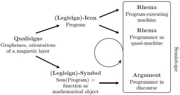
We rely on Bense’s collection of semioses [12, p. 45ff]. There, 25 examples of 27 classes of meaning are listed. A 26th example is the semiosis (legisign)-icon \(\to\) rhema in the diagram, which just indicates the neither-true-nor-false of the interpretant entity scanning the icons, be it machine, enzyme, or human. With the (legisign)-symbol, it is convenient to consider the Scottian semantic map as a whole as the object reference of the program-qualisigns.
The difference between the top and the bottom is that between the programmer as craftsman and the programmer as thinker. Composed in semioses: Quali \(\to\) (Legi)-Icon \(\to\) Rhema versus Quali \(\to\) (Legi)-Symbol \(\to\) Argument. This brings to mind my experimental physics professor, who said to us at the beginning of our studies: “Not every radio hobbyist is compelled to be a physicist!” The lower half of the diagram opens the door to mathematical argumentation and thus to further knowledge about programs and program equivalences (symmetries), and as a result to multiplicatively better mastery, such as intelligent word processing.
With this, a second Hilbertian tradition comes into play, which Max Bense summarized in [12, p. 157] as follows: “Hilbert expressly raised as a methodical requirement the consistency of the concluding clauses of a proof. This indicates the fact that the semiosis of increasing semioticity that is introduced and characteristic of the generation of a proof must not become a retrosemiosis of falling semioticity in any phase of the deductive construction in achieving an argument. If this were to happen, then the purely intellectual process of ‘thirdness’ would fall back into ‘secondness’ or ‘firstness’.” In the same way, Scott’s calculus safeguards against the catastrophe of chaotically cobbled-together programs.
The third semiosis of our diagram only makes sense together with a fourth, namely the subsumption of all interpretants into a sign that seems to me so formidable that I would like to call it a semiotope — by analogy to a biotope. Incidentally, for this semiotope to be consistent, the machine processing a Scott-reflected language also formally does what the programs demand. (See our mini-language in §2, which still lacks a command for text concatenation, but the reader can easily figure it out.) Incidentally, the proof of consistency can be performed within the framework of non-standard semantics (see [3]).
The looping-arrow semiosis in the diagram takes the programmer from acting on the icon-programs to contemplating them.
7. Extension into Semiotics - A Follow-up
Similar to René Thom, Scott opens up new approaches to exact thinking about becoming (see e.g. [14]). Just as the work of the Stuttgart Semiotics Center also makes use of Thom’s theory, it would likely be fruitful to pursue the semiotics of Scott’s semantics further — all under the keyword ‘process’. Rich encouragement can be found in the Semiosis issues of recent years. Think of Bense’s summary [15]: “The semiotic representation of a system of theoretically connected or connectible entities, i.e. of a theory or discipline, is always realized in a certain set of sign classes or trichotomies (thematics of realization) of the complete sign.”
Here the complete Scottian sign is probably always given by two text levels, as they are typically e.g. occur in the second equation of §5 (the ‘g’ after the “while B do C”) — see also the papers [16] and [17] by Marty and Walther. The reference of our diagram to those in [18] would have to be established — plunging ever further into its references to Lawvere. Word processing programs belong to word and formula languages at the same time [19]. Finally, it is significant in this connection that Max Bense keeps coming back to the topic of functionality ([20]), which is so closely related to the concept of communication channels for processing data.
Bibliography
- Scott, D. (1970). “Advice on modal logic,” in Lambert, K. (Ed.). (1970). Philosophical Problems in Logic: Some Recent Developments. Dordrecht: D. Reidel Publiching Co., pp. 143-73
- Scott, D. & Strachey, C. (1971). “Toward a Mathematical Semantics for Computer Languages,” in Fox, J. (Ed.). (1971). Proceedings of Symposium on Computers and Automata. New York.
- Stoy, J. (1977). Denotational Semantics: The Scott-Strachey Approach to Programming Language Theory. Cambridge, MA: MIT Press.
- Milne, R. & Strachey, C. (1976). A Theory of Programming Language Semantics, Parts A and B. New York: Halsted Press
- Wagner, E. (1971). “An Algebraic Theory of Recursive Definitions and Recursive Languages.” Proceedings of the 3rd ACM Symposium on Theory of Computing, pp. 12-23
- Scott, D. (1972). “Lattice Theory, Data Types and Semantics,” in Rustin, R. (Ed.). (1972). Formal Semantics of Algorithmic Languages. Englewood Cliffs, NJ: Prentice-Hall, pp. 65-106
- Scott, D. (1976). “Data Types as Lattices.” SIAM Journal on Computing 5(3), pp. 522-87
- Scott, D. (1971). “The Lattice of Flow Diagrams,” in Engeler, R. (Ed.). (1971). Symposium on the Semantics of Algorithmic Languages. Berlin: Springer-Verlag, pp. 311-66
- Scott, D. (1977). “Logic and Programming Languages.” Communications of the ACM 20(9), pp. 634-41
- Tarski, A. (1955). “A Lattice-theoretical Fixpoint Theorem and its Applications.” Pacific Journal of Mathematics 5(2), pp. 285-309
- Nees, G. (to appear). “M. Bense’s Esthetics and D.S. Scott’s Theory of Information.” Semiosis. [editor’s note: this was never published]
- Bense, M. (1975). Semiotische Prozesse und Systeme. Baden-Baden: Agis-Verlag.
- Hilbert, D. (1926). “Über das Unendliche.” Mathematische Annalen 95, pp. 161-90
- Thom, R. (1978). “Vom Icon zum Symbol.” Semiosis 10, pp. 5-23
- Bense, M. (1978). “Zeichenklassen und mathematische Grundbegriffe. Semiosis 11, pp. 72-4
- Marty, R. (1978). “L’ideologie comme processus semiotique.” Semiosis 11, pp. 55-66
- Walther, E. (1978). “Notiz zur Frage des Zusammenhangs der Zeichenklassen.” Semiosis 11, pp. 67-71
- Bense, M. (1976). “Semiotische Kategorien und algebraische Kategorien.” Semiosis 4, pp. 5-19
- Bense, M. (1977). “Wortsprache und Formelsprache.” Semiosis 8, pp. 53-7
- Bense, M. (1979). “Die funktionale Konzeption der Semiotik.” Semiosis 13, pp. 17-28